
Introduction
Before I start with our prediction model on USA housing prices, I just want to thank Aurélien Géron for his book : Hands-On Machine Learning with Scikit-Learn and TensorFlow: Concepts, Tools, and Techniques to Build Intelligent Systems 1st Edition.
The book is available on Github for free. You can view it here.
Get and look at the data
I will use some of what I learned.......or copied :-) from chapter 2 of this book to create a prediction model. The model is going to be trained on the USA housing data. You can download the data here.
Once you have downloaded the data it is time to read in the data. Lets write a function to read in the data.
import pandas as pd
import numpy as np
import os
HOUSING_PATH = "datasets\\USA_Housing\\"
FILE_NAME = "USA_Housing.csv"
def load_data(housing_path = HOUSING_PATH, file_name = FILE_NAME):
csv_path = os.path.join(housing_path, file_name)
return pd.read_csv(csv_path)
housing = load_data()
Let's have a look at the data.
print(housing.head())
Avg. Area Income Avg. Area House Age Avg. Area Number of Rooms \
0 79545.458574 5.682861 7.009188
1 79248.642455 6.002900 6.730821
2 61287.067179 5.865890 8.512727
3 63345.240046 7.188236 5.586729
4 59982.197226 5.040555 7.839388
Avg. Area Number of Bedrooms Area Population Price \
0 4.09 23086.800503 1.059034e+06
1 3.09 40173.072174 1.505891e+06
2 5.13 36882.159400 1.058988e+06
3 3.26 34310.242831 1.260617e+06
4 4.23 26354.109472 6.309435e+05
Now lets check the summary of columns count and data types of the DataFrame.
print(housing.info())
RangeIndex: 5000 entries, 0 to 4999
Data columns (total 7 columns):
# Column Non-Null Count Dtype
--- ------ -------------- -----
0 Avg. Area Income 5000 non-null float64
1 Avg. Area House Age 5000 non-null float64
2 Avg. Area Number of Rooms 5000 non-null float64
3 Avg. Area Number of Bedrooms 5000 non-null float64
4 Area Population 5000 non-null float64
5 Price 5000 non-null float64
6 Address 5000 non-null object
The DataFrame is made up of 5000 rows. Luckily for us we have no missing values. We also see that all of the columns contain numbers(floats) except the "Address" column.
The median income or average income is usually the main indicator for housing prices. We have an "Avg. Area Income" column in the DataFrame. Let's create a category by using the "Avg. Area Income" column.
# This will turn the labels into integers instead of floats
housing["income_cat"] = pd.cut(housing["Avg. Area Income"],
bins=[0, 40000, 60000, 80000, 90000, 110000],
labels=[1, 2, 3, 4, 5])
print(pd.cut(housing["Avg. Area Income"],
bins=[0, 40000, 60000, 80000, 90000, 110000]).value_counts())
print(housing["income_cat"].value_counts())
Below it shows how the data is split by average income. Then it shows how the data is split into the 5 categories. So category "5" shows 102 areas that have an average income between USD 90,000 and USD 110,000.
(60000, 80000] 3272
(40000, 60000] 1019
(80000, 90000] 588
(90000, 110000] 102
(0, 40000] 19
Name: Avg. Area Income, dtype: int64
3 3272
2 1019
4 588
5 102
1 19
Name: income_cat, dtype: int64
Create a train and test set for our prediction model
It is good practice to set aside a test set and not look at it. If we don't then we may fall prey to data snooping. I got the simplest explanation on data snooping from quantitrader.com .On their website is says "Data snooping refers to statistical inference that the researcher decides to perform after looking at the data".
Since we have 5 categories in our data it is important that we draw out samples in proportion to those categories. This is referred to as stratified sampling. It means that the sample should be representative of the overall population. The below shows how the data is split by percentage between the 5 categories.
print(housing["income_cat"].value_counts() / len(housing) *100)
Name: Avg. Area Income, dtype: int64
3 65.44
2 20.38
4 11.76
5 2.04
1 0.38
Name: income_cat, dtype: float64
From the above we see that category 3 represents most of the population with 65.44%. Now lets do some stratified sampling.
split = StratifiedShuffleSplit(n_splits=1,test_size=0.2, random_state=42)
for train_index, test_index in split.split(housing,housing["income_cat"]):
strat_train_set = housing.loc[train_index]
strat_test_set = housing.loc[test_index]
# Drop the 'income_cat' so that the data is back to its original state
for set in (strat_train_set,strat_test_set):
set.drop(["income_cat"],axis=1,inplace=True)
Visualize data to gain insights
Before we start lets create a copy of our training set.
housing = strat_train_set.copy()
Let's see how much each attribute(column) correlates with the "Price"
corr_matrix = housing.corr()
print(corr_matrix["Price"].sort_values(ascending=False))
Price 1.000000
Avg. Area Income 0.641284
Avg. Area House Age 0.453640
Area Population 0.407540
Avg. Area Number of Rooms 0.335065
Avg. Area Number of Bedrooms 0.167008
Name: Price, dtype: float64
As mentioned earlier,median income or average income is usually the main indicator for housing prices. By looking at the above correlations it shows that indeed "Avg. Area Income" has the best correlation to the "Price".
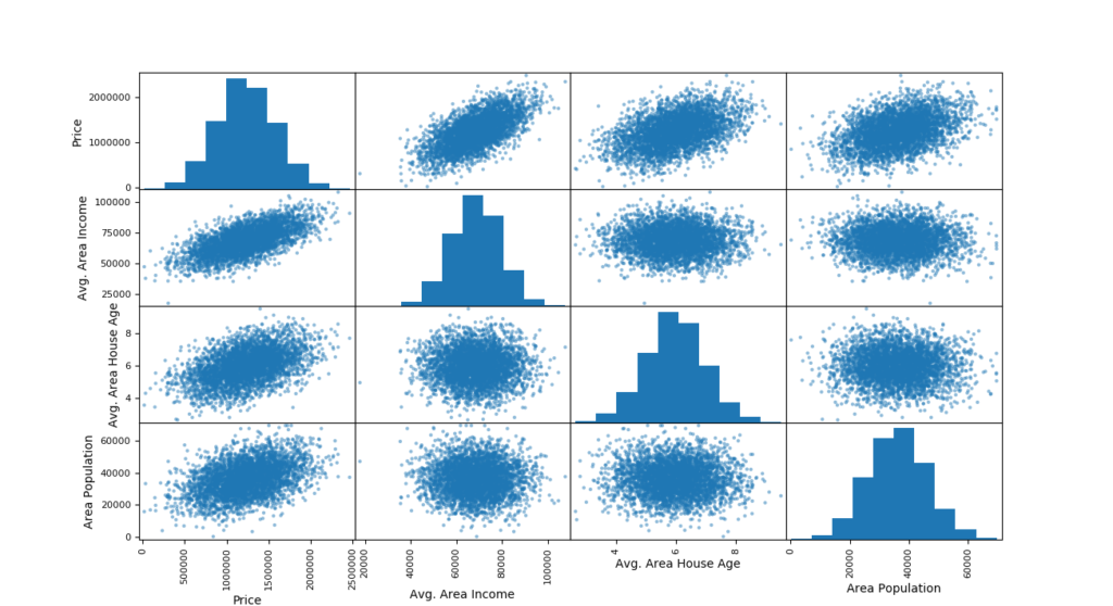
We can visualize how the 3 top attributes correlate with the house price via a scatter matrix.
import matplotlib.pyplot as plt
attributes = ["Price", "Avg. Area Income", "Avg. Area House Age", "Area Population"]
pd.plotting.scatter_matrix(housing[attributes],figsize=(12,8))
plt.show()
Now we can zoom in to the "Avg. Area Income" and "Price" since it shows the most promise.
housing.plot(kind="scatter", x="Avg. Area Income", y="Price", alpha=0.5)
plt.show()
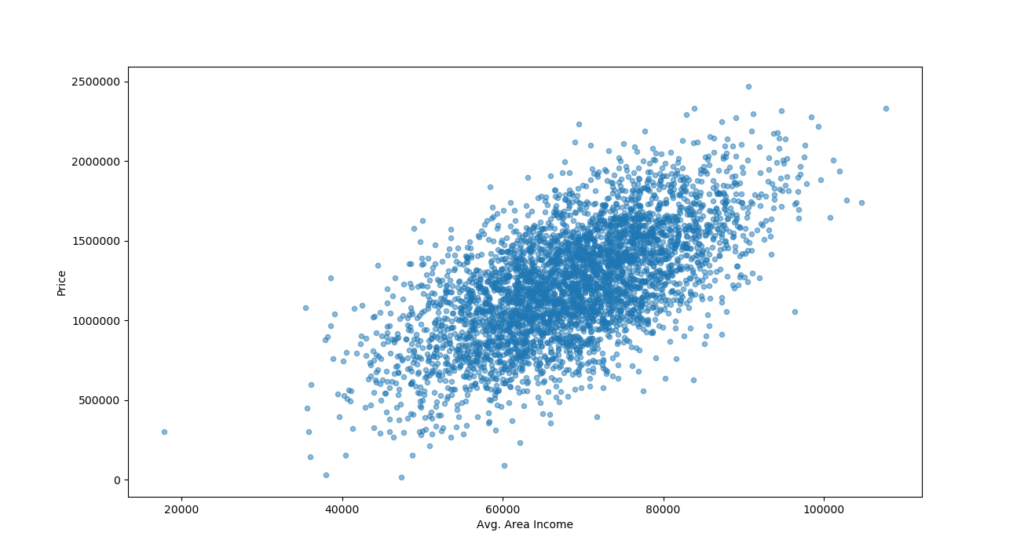
The above reveals a strong correlation as the points are not too dispersed. We can use the Avg. Area Income in our prediction model to determine the house prices.
Prepare data for the machine learning algorithm
First we need to separate the predictors and the labels because we do not want to apply the same transformations to them
housing = strat_train_set.drop("Price", axis=1)
housing_labels = strat_train_set["Price"].copy()
We do not have any missing data in our DataFrame. But you might get another data set that has missing values. Therefore we need to account for that missing by using Scikit-Learn's Imputer.
from sklearn.imputer import SimpleImputer
imputer = SimpleImputer(strategy="median")
housing_num = housing.drop("Address",axis=1)
imputer.fit(housing_num)
All we are saying here is that if we encounter a missing value, we want to replace that missing value with the median value. We can check to see if the median value is indeed being used be executing the below code.
print(imputer.statistics_)
print(housing_num.median().values)
[6.87638750e+04 5.95444768e+00 7.01010359e+00 4.05000000e+00
3.60921720e+04]
[6.87638750e+04 5.95444768e+00 7.01010359e+00 4.05000000e+00
3.60921720e+04]
Both results are the same which is what we wanted. Now we can use the trained imputer to transform the training set by replacing the missing values by the learned medians. This won't do anything for this data set because it has no missing values but it will be very handy for data sets with missing values.
# Returns a Numpy array
X = imputer.transform(housing_num)
# Turn the array into a Pandas DataFrame
housing_tr = pd.DataFrame(X,columns=housing_num.columns)
Let's now build a small pipeline. The pipeline in the Hands on ML book is bigger than what we are going to do here. The Pipeline class helps to execute the data transformation steps in the right order. We will also include scaling in our data using Scikit-Learn's StandardScalar.
from sklearn.pipeline import Pipeline
pipeline = Pipeline([
("imputer", SimpleImputer(strategy="median")),
("std_scaler", StandardScaler()),
])
housing_tr = pipeline.fit_transform(housing_num)
Select and Train a model
I found out though practice(the few models I built) and by listening to Dr Eugene Dubossarsky that the RandomForestRegressor is best most cases. Because of this I'm not going to show how different models compare with each other. So let's create a model, fit it and get save some prediction and actual values.
from sklearn.ensemble import RandomForestRegressor
my_model = RandomForestRegressor()
my_model.fit(housing_tr, housing_labels)
# Get some data and some labels. That last 10 instances
some_data = housing_num.iloc[:10]
some_labels = housing_labels.iloc[:10]
some_data_prepared = pipeline.transform(some_data)
Now let's calculate some indicators like MSE(mean squared error) and RMSE(root mean squared error).
from sklearn.metrics import mean_squared_error
housing_predictions = my_model.predict(housing_tr)
my_model_mse = mean_squared_error(housing_labels,housing_predictions)
my_model_rmse = np.sqrt(my_model_mse)
print("Model Root Mean Squared Error:", my_model_rmse)
Model Root Mean Squared Error: 44638
The price range of a house is between USD15,938 and USD2,469,065 which is huge. The RMSE is equal to USD44,638 which means a typical prediction error will be around USD44,638. Is the RMSE to big? I don't think so but lets use cross validation before we predict and then see.
from sklearn.model_selection import cross_val_score
my_model_scores = cross_val_score(RandomForestRegressor(),
housing_tr,housing_lables,scoring="neg_mean_squared_error",cv=10)
my_model_rmse_scores = np.sqrt(-my_model_scores)
def display_scores(scores):
print("Mean: ", scores.mean())
print("Standard deviation: ", scores.std())
display_scores(my_model_rmse_scores)
Mean: 119997
Standard deviation: 4704
We get standard deviation of US4,704 . Is that good or bad? I think it's good.
Predictions
Finally we can do some predictions and compare with actual prices
# Set prediction price and actual price variables
predictions = np.ceil(my_model.predict(some_data_prepared))
actuals = np.ceil(list(some_labels)
for p, a in list(zip(predictions, actuals)):
percentage_diff = (a - p) / a * 100
percentage_diff = round(percentage_diff,2)
print("Prediction:", int(p), "Actual:", int(a), "Percentage difference:", percentage_diff)
Prediction: 1465430 Actual: 1430797 Percentage difference: -2.42
Prediction: 1085427 Actual: 1063070 Percentage difference: -2.1
Prediction: 1684467 Actual: 1675703 Percentage difference: -0.52
Prediction: 1060784 Actual: 1025418 Percentage difference: -3.45
Prediction: 920581 Actual: 971100 Percentage difference: 5.2
Prediction: 940129 Actual: 960905 Percentage difference: 2.16
Prediction: 846154 Actual: 778837 Percentage difference: -8.64
Prediction: 760471 Actual: 771311 Percentage difference: 1.41
Prediction: 972058 Actual: 974600 Percentage difference: 0.26
Prediction: 1153677 Actual: 1185227 Percentage difference: 2.66
The percentage difference is ranges between -8.7% to 5.2% which comes to a 13.9% variance. Is it good? I think so again. Maybe you can build a better one. Maybe I missed something that you can see and improve on. If so, go for it!
I hope this post could help you to build a not so simple model. I'll see you in the next post.