Introduction

Welcome to part 4th of this series. We will focus on Chapter 8:The Central Limit Theorem. There are many technical definitions online for the central limit theorem, but Chalers Wheelan explains it simply in one sentence.“The core principle underlying the central limit theorem is that a large, properly drawn sample will resemble the population from which it is drawn”-Page 128.

We will still stick to our hockey data set. I suggest you start at part1 of this series for better understanding of what is about to follow.

Sample means

From our underlying population we can draw 100 samples of 20 players per sample and 100 samples of 100 players per sample. Then we can calculate the means for each of those samples.

Height

The mean height for our hockey player data set was 182.04cm. Let us graph our two sample means and see how that compares to our population mean.‍

‍

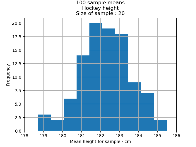
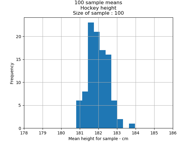
The larger the sample size the more likely that the samples means are clustered tightly around the mean of the underlying population. This is in line with the central limit theorem which tells us that a large sample will not typically deviate from its underlying population(hockey data set).

From the two charts we can observe a tighter cluster around the population mean(182.04cm) of the sample size of 100. The 1st chart(Size of sample: 20) shows that to sample means are more dispersed than the 2nd chart.

Weight

The mean weight for our hockey player data set was 83.74kg. Let’s again graph our two sample means and see how that compares to the mean of our underlying population.

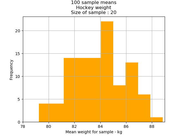
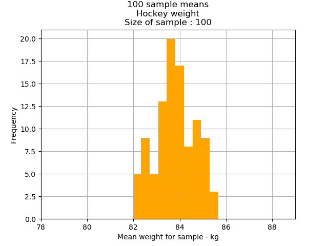
The findings are the same. The sample means of the larger sample size(2nd chart) are clustered more tightly around the original population mean of 83.74kg than the sample means of the smaller sample size(1st chart).

The standard error explained

While the standard deviation is a number that shows the dispersion around the population mean, the standard error measures the dispersion around the sample means. A large standard error means that the sample means are more spread out around the population mean.

The formulafor standard error is:

StandardError = s / √n

s = Standard deviation of the population

n = Number of the sample size

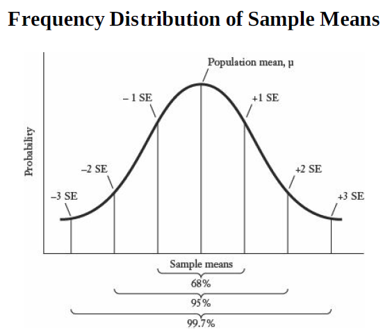
Just like the standard deviation, we can expect that roughly

68 percent of all sample means will lie within one standard error of the population mean;

95 percent of the sample means will lie within two standard errors of the population mean; and

99.7 percent of the sample means will lie within three standard errors of the population mean.

‍

The standard error calculations

Lets solve for the standard errors for height and weight.

Height

From previous posts our standard deviation for height was 5.87.

Sample size: 20

Standard Error = s / √n

Standard Error = 5.87 / √20

Standard Error = 5.87 / 4.472135955

Standard Error = 1.31

68 percent of all sample means are between 180.73cm and 183.35cm;

95 percent of the sample means are between 179.42.cm and 184.66cm; and

99.7 percent of the sample means are between 178.11cm and 185.97cm.

Sample size: 100

Standard Error = s / √n

Standard Error = 5.87 / √100

Standard Error = 5.87 / 10

Standard Error = 0.587

68 percent of all sample means are between 181.45cm and 182.63cm;

95 percent of the sample means are between 180.87.cm and 183.21cm; and

99.7 percent of the sample means are between 180.28cm and 183.80cm.

So can see this by just looking at the charts.

Weight

The standard deviation for weight was 8.55.

Sample size: 20

Standard Error = s / √n

Standard Error = 8.55/ √20

Standard Error = 8.55 / 4.472135955

Standard Error = 1.91

68 percent of all sample means are between 81.83kg and 85.65kg;

95 percent of the sample means are between 79.92.kg and 87.56kg; and

99.7 percent of the sample means are between 78kg and 89.48kg.

‍Sample size: 100

Standard Error = s / √n

Standard Error = 8.55 / √100

Standard Error = 8.55 / 10

Standard Error = 0.855

68 percent of all sample means are between 82.89kg and 84.60kg;

95 percent of the sample means are between 82.03.kg and 85.45kg; and

99.7 percent of the sample means are between 81.18kg and 86.31kg.

Again, you can see this by just looking at the charts.

In our next and possibly final post of this series we will include the NBA data set. Hope you enjoyed it. See you in the next post.